
Introduction
The small organisms that live at the bottom of the marine life food chain, phytoplankton, are more important than we think. Their main purpose involves absorbing CO2 from our atmosphere and using it as a nutrient to promote growth in existing populations, while in turn, producing oxygen that us humans need in order to breathe. But, why should we care about these microscopic creatures? CO2 has been increasing due to human activity of burning fossil fuels (especially in car emissions) and land use changes such as deforestation transpire. Our phytoplankton absorb up to 30% of CO2 and through dissolving it into the ocean, multiple series of chemical reactions occur in which the overall quantity of hydrogen ions increases. This is detrimental to our largest water source as the hydrogen ions contribute to acidification, or decreasing the pH of the ocean and affecting the ecosystems within it. Currently, the ocean’s pH is 8.1, a 0.1 difference from pre-industrial era, suggesting its slow decline. However, by 2100, the ocean’s pH is expected to drop to 7.67 (NOAA).
Among CO2, there are other important nutrients that enable phytoplankton to grow, such as nitrates, silicates, carbonates, iron, and sunlight. However, just while CO2 is as beneficial as it is disadvantageous, another element exists as a nutrient while also threatening phytoplankton if bioavailability and toxicity increases: copper. As a pollutant, this metal and its concentration are expected to increase by 115% over the next century. The sources of copper in the ocean are minerals in the soil and weathered rock which form sediments and suspended particles in the water, extraction of copper from rock into a dissolved state, biological particles and systems that heat the ocean, like volcanic action (Blossom). While copper is great for phytoplankton growth, high and low levels of copper concentrations can be detrimental. In response to this, we created an experiment in which we attempt to determine the range of copper concentration that diminishes phytoplankton in acidic environments as the ocean is undergoing acidification. Our chosen species of phytoplankton is Thalassiosira weissflogii, or T.weiss for short. We hypothesize that additional copper and a slightly acidic pH which is a direct result of ocean acidification will elevate the toxicity of copper in T.weiss by 2100.
Methods
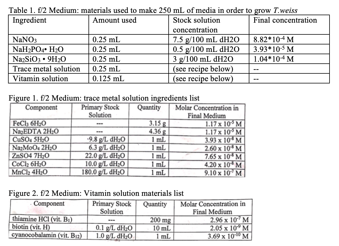
In order to grow our cultures, we followed the f/2 Medium created by Guillard in 1975. In addition to the medium’s ingredients listed in the table below, we used 250 mL of sterile water and 8 mL of instant ocean salt to create a saline, marine environment along with relatively 100 mL of previously gathered T.weiss by our professor, Dr. De Haan. Mixing the solution together by shaking vigorously, we used this method to create three different cultures of phytoplankton. Our vitamin and trace metal solutions were pre-made; however, their ingredients are listed below in figures 1 and 2.
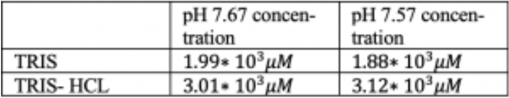
In order to create an acidic environment of pH 7.57 or pH 7.67, we created buffer solutions using Tris and Tris+HCl. Their target concentrations are described in figure 3 below. We used 0.4741 g of Tris + HCl and 0.2430 g of Tris for pH of 7.67. We added these grams to 10 mL volumetric flasks in which we quantitatively added the Tris + HCl to one flask and the Tris to another flask, then filling the rest of the flask to the indicated line with distilled water. Then, we added roughly 0.2 mL of each to our solutions that were indicated as acidic and added 0.2 mL of distilled water to solutions indicated as normal pH. For the pH of 7.57, we determined that 0.4917 g of Tris + HCl would need to be used and 0.2282 g of Tris would be used in order to create the acidic environment we desired.
Figure 3. Target concentrations of Tris and Tris + HCl for pH of 7.57 and 7.67
The equation used to determine the correct amount of Tris and Tris + HCl we needed to create our targeted pH’s is shown below in figure 4.

The values for x were found in mM which we converted to M in 10 mL, then solving for the grams of both Tris and Tris + HCl we needed to add to the solutions that were indicated as acidic.
Figure 5. Color scale of phytoplankton exhibiting cell growth amounts
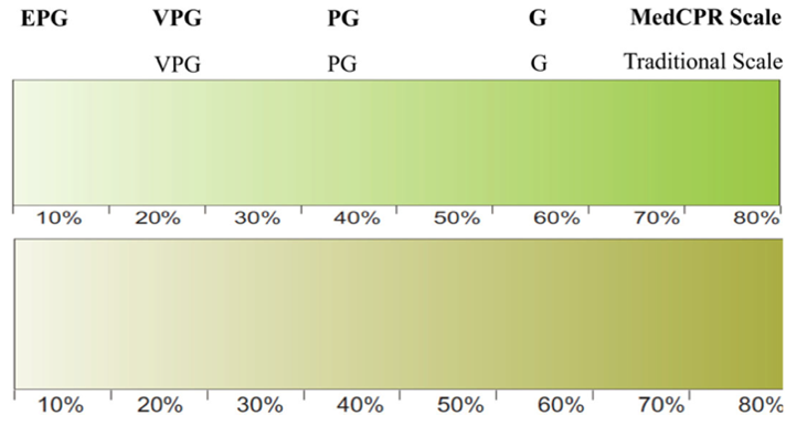
This figure shows the color scale used when assessing the color change of the phytoplankton every other day. The traditional scale—the scale below the more lime green scale—was the one the phytoplankton cultures were compared to. Higher cell growth accounted for a darker color, while slow-to-none cell growth is represented by a lighter color. This scale was used for all three cultures.
Culture 1:
Table 2. Copper concentrations used for four groups of phytoplankton for Culture 1

Note in the f/2 recipe, 0.0393 uM of stock copper solution is already used. Therefore, we determined this as our control group and did not add any excess copper. The rest of the three groups involved diluting the copper stock solution by factors of 10 in which the copper solution we used had a mM of 15.7, shown in Table 1 and the copper included in the original f/2 medium had a molar concentration of 3.93×10⁻⁸.
Culture 2:
Table 3. List of solutions made for the second culture of phytoplankton
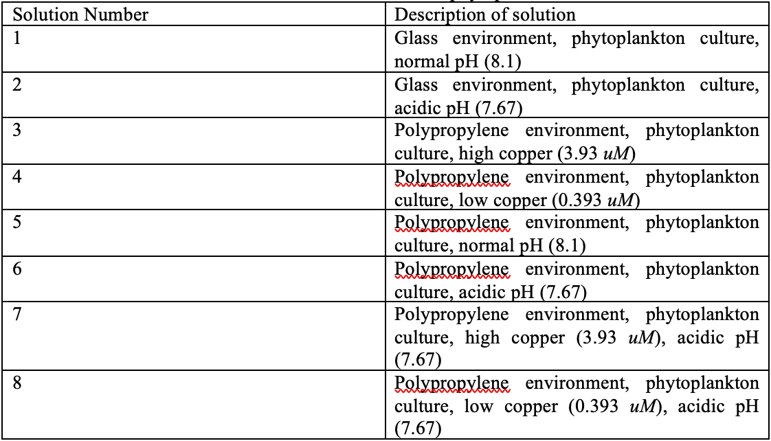
As this culture reflects our factorial experiment, we made sure to include multiple varieties of samples that related to our two factors in our factorial method (environment and acidity), while also testing the effects of low or high copper concentrations have on phytoplankton growth. The environment refers to whether the phytoplankton was grown in glass or plastic (polypropylene) vials. Copper was not included in our factorial grid, and therefore our results seen in the graphs offer conclusions not found in our factorial experiment.
Table 4. Factorial Experiment for Culture 2, after 7 days

Table 5. Calculating variation in the factorial experiment of culture 2 data
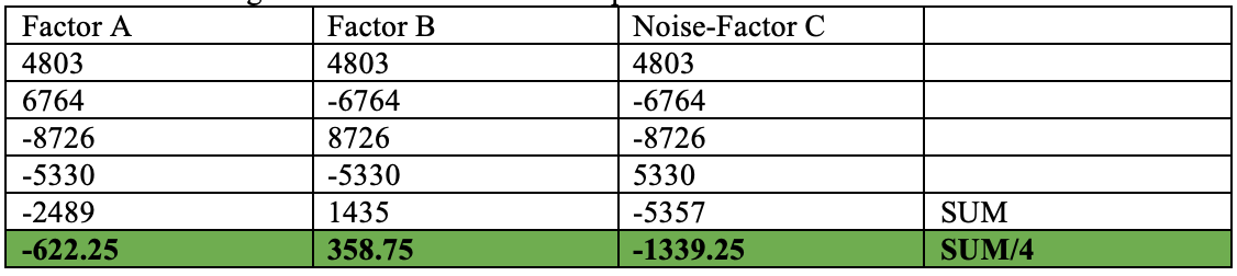
The bolded numbers in the last row of this data set shows the response factors and how significant each factor is on phytoplankton growth. As you can see, the most different value from zero is factor “C,” or “noise” which means that C has the most significant impact on the growth of T.weiss. In contrast, factor “B”, or the environment the phytoplankton grows in, is virtually not too far off from zero, so we can assume that it has little to no effect phytoplankton growth.
Culture 3:
Table 6. List of solutions made for the third culture of phytoplankton
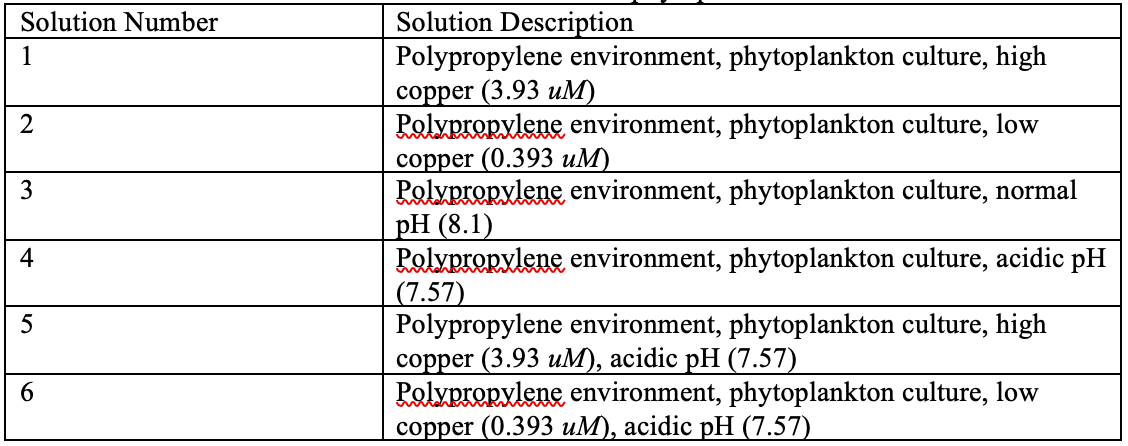
Like culture two, culture three involves samples that have either high Cu, low Cu, acidity, or normal pH values—or a combination of two factors. This corresponds to our factorial experiment as we test the effects of acidity and Cu concentrations on our cultures, this time with a pH 0.10 lower than that of culture two.
All three cultures:
In addition to the color scale we used to observe whether our phytoplankton cultures were growing, we also used a Coulter counter. The principle of a Coulter counter institutes that particles pulled through an opening, along with an electric current, produce a change in electrical resistance that is proportional to the volume of the particle going through the opening. We first diluted our samples by obtaining 2 mL of each solution with either an automatic pipet or a 1 mL standard pipet and then transferred the 2 mL into the plastic container meant to hold samples tested in the instrument. We then filled the rest of the plastic containers to the 20 mL marker with 18 mL of Isoton as that is the accepted diluent—a fluid that dilutes—for the counter. This dilution process was used for testing all three of our cultures with a ratio of 18 mL of Isoton for every 2 mL of solution. Therefore, the use of this instrument was key in our research as it analyzed the number of particles or cells that were growing in each culture and depicted any changes, such as dying populations which could not be physically seen through the color change observations using the scale.
Results:
Culture 1:
Figure 6. T.weiss Culture 1 Number of Days of Growth vs. Color Scale (%) Observed
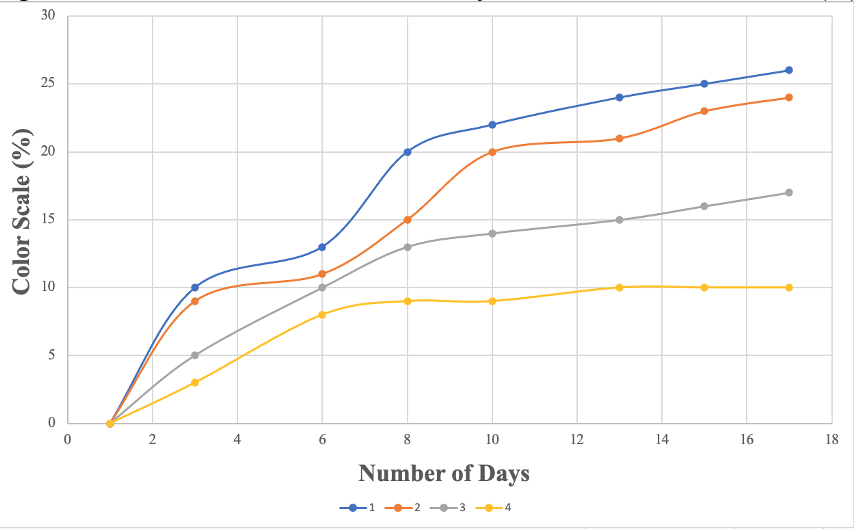
The graph shows how our control group, group 1, had the most growth, which was expected as no external factors were added. Color scale is rather unreliable here; however, what we can conclude from this graph is that the highest Cu concentration of 39.3 uM had the most impact of cell growth, as seen by the line being the shallowest curve (group 4, in yellow).
Table 7. T.weiss Culture 1 Number of Days of Growth vs. Cell Count (um) (averages)
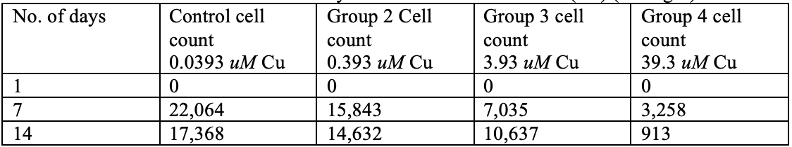
Notice how group 4 grew the least and also decreased in cell count to the smallest population of just under one thousand in comparison to the other three groups which remained in the ten thousands range. Overall, this data does not explicitly tell us what copper concentrations are the most detrimental as the result varied. Group 3, the second to least diluted copper concentration had continued to grow after the fourteen day experiment, offering inconclusive evidence of whether this range of copper concentrations is the exact threshold able for T.weiss to grow in.
Culture 2:
Figure 7. T.weiss Culture 2 Number of Days of Growth vs. Color Scale (%) Observed
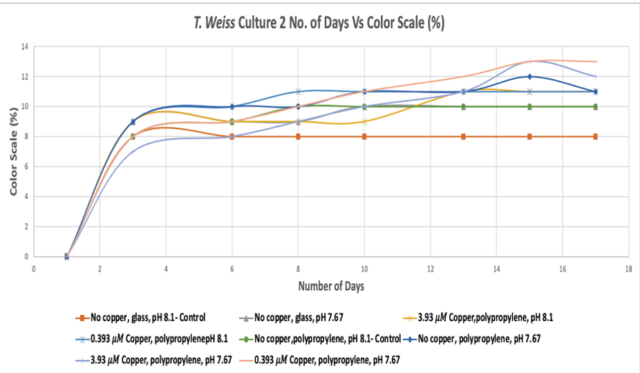
The orange line, depicting our control group which had no additional copper added to it, had the least overall growth in terms of color change. The other groups, however, continue to overlap and intertwine, making it difficult to directly tell whether copper, acidity, or the environment of our phytoplankton affected its growth. Therefore, let’s look below at our cell count data.
Table 8. T.weiss Culture 2 Number of Days of Growth vs. Cell Count (um)
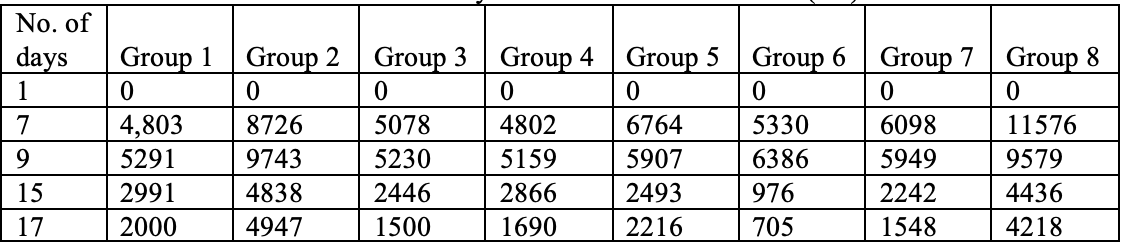
Notice how group 8 (Polypropylene environment, phytoplankton culture, low copper (0.393 uM), acidic pH (7.67)) began with the largest cell count, but did not end with the largest cell count at the seventeenth day mark. This table also shows that the difference between groups aside from their components is hard to decipher as all grow at similar rates but begin to die off at similar times (around day 9 onward). What is interesting is group two (Glass environment, phytoplankton culture, acidic pH (7.67)) is the only group to begin to deplete towards day 15, but slowly grow again. This, however, does not tell us anything about whether the specific acidity of pH of 7.67 is detrimental to our phytoplankton, motioning us to refer to the conclusions of the factorial experiment above.
Culture 3:
Figure 8. T.weiss Culture 3 Number of Days of Growth vs. Color Scale (%) Observed
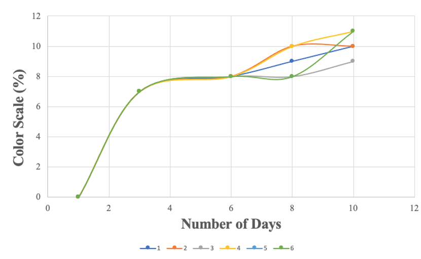
As culture three was the newest-made population of phytoplankton, this graph only shows the data from the first ten days. As we found through background research that phytoplankton tends to have about a week-and-a-half long growth period until the cell count plateaus, it makes sense that the curves, aside from group two and group five, continue to increase upwards.
Table 12. T.weiss Culture 3 Number of Days of Growth vs. Cell Count (um)
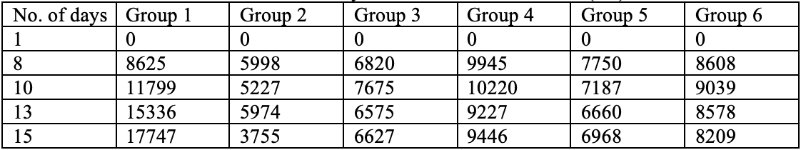
What is most interesting about the data from this table is that after our culture three begins to die off and decrease in cell count in all groups around the span between day 10 and 13 (except group 1 and 2), they begin to increase their cell count after day 13. What is also intriguing is how group 4 has the largest cell growth at the beginning (day 8-after one week), but it was the solution that contained a polypropylene environment and acidic pH (7.57) along with our phytoplankton culture—but, this solution did not include any additional copper. We hypothesized that a lower pH (more acidic environment) would have an impact on the phytoplankton growth, but the relatively high cell count at the beginning suggest that it may not be that effective as we thought. Group 1 is also eye-catching in that it is the only group that did not “die off” or decrease in cell count at any point during the fifteen-day experiment. This is interesting because group 1 had a high concentration of Cu (3.93 uM).
Discussion:
As our factorial experiment indicates, the noise factor was the most significant towards affecting phytoplankton growth in that the negative condition helped resulting in the slowing of growth rate. The least significant factor was the glass versus propylene environment in that there was little to no effect on the cell growth. The magnitude of C’s value, -1339.25, tells us that the phytoplankton growth that we measure is relatively affected by the “noise,” which in this case goes against our hypothesis in that we believed the acidity of the environment would affect the growth the most. In comparison, factor A’s magnitude of -622.25 tells us that the cell counts we measure in acidic environments are the second most significant response factor. Furthermore, as examined previously, factor B, or glass versus polypropylene environments, has little to no effect on phytoplankton growth as it has the smallest magnitude.
Our graphs and tables of data are rather inconclusive in that our hypothesis was neither disproven nor proven as the results are varying in whether or not acidity is at fault or copper concentration is at fault for the growth and then dying of our cultures. Therefore, our unanswered question of establishing the threshold for how much copper our phytoplankton species can handle in terms of its detrimental effect of slowing and decreasing cell growth was not determined in our experiment. What we can admit to is that as the concentrations of copper used increase, the rate at which the phytoplankton’s growth plateaus and then dies off increases, noted as such by the 39.3 uM having the least cell growth and smallest cell count over the fourteen day period in culture 1 (depicted as group 4).
Figure 9. Pressure CO2 at pH of 7.67
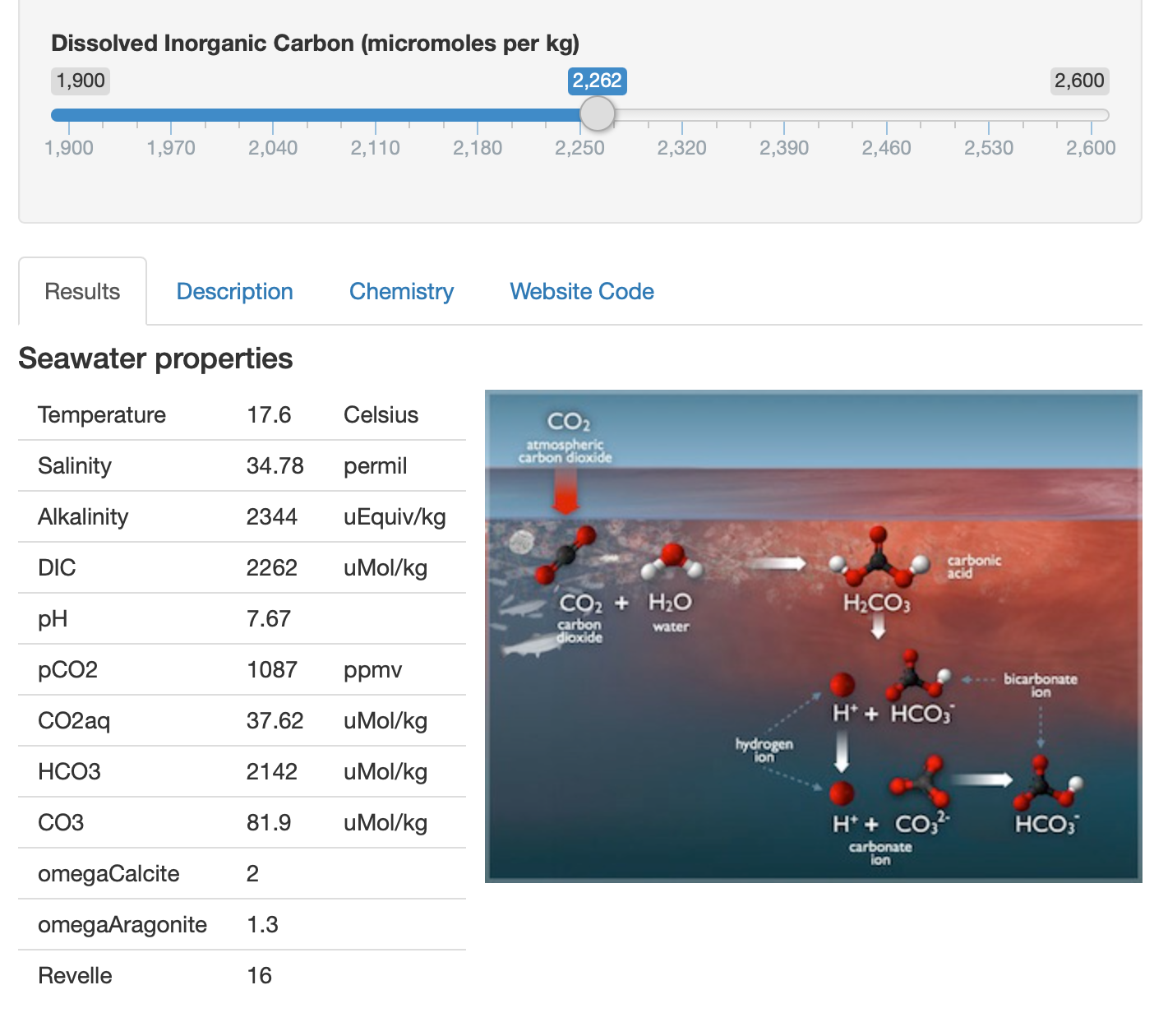
The DIC or dissolved inorganic carbon needed for the pH to be at 7.67 in the year 2100 is exhibited as 2,262 umol/kg and the pressure of CO2 is calculated as 1087 ppmv.
Figure 10. Pressure of CO2 at pH of 7.57
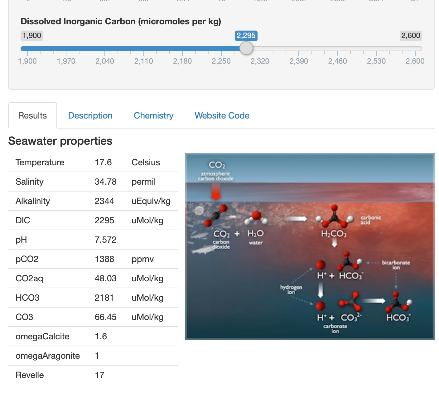
The DIC or dissolved inorganic carbon needed for the pH to be at 7.57 in the year 2100 is exhibited as 2,295 umol/kg and the pressure of CO2 is calculated as 1388 ppmv.
As the pH of the ocean will continue to decrease as climate change affects the production of our carbon dioxide absorbing phytoplankton, the likelihood that these higher pressures of CO2 depicted in figures 9 and 10 will be up-taken by our small organisms is slimming as the quantity is steadily and exponentially increasing in relation to how fast the phytoplankton can grow. Therefore, it is our job to recognize that climate change not only puts humans at risk, but even the smallest creatures in our ecosystems are impacted as well. As phytoplankton help increase the amount of accessible oxygen to our population, it is important for us to protect their populations that are at risk from harmful pollutants like copper and excess of carbon.
References
Barton, A., Irwin, A., Finkel, Z., & Stock, C. (2016, March 15). Anthropogenic climate change drives shift and shuffle in North Atlantic phytoplankton communities. Retrieved March 23, 2021, from https://www.pnas.org/content/113/11/2964
Evans, Monica. “Climate Fix? ‘Fertilizing’ Oceans with Iron Unlikely to Sequester More Carbon.” Mongabay Environmental News, 22 May 2020, news.mongabay.com/2020/03/climate-fix-fertilizing-oceans-with-iron-unlikely-to-sequester-more-carbon/.
NOAA. “What Is Ocean Acidification?” National Ocean Service, 26 Feb. 2021, oceanservice.noaa.gov/facts/acidification.html.
Santos, Carmen B. de los, et al. “Interaction of Short-Term Copper Pollution and Ocean Acidification in Seagrass Ecosystems: Toxicity, Bioconcentration and Dietary Transfer.” Marine Pollution Bulletin, vol. 142, 2019, pp. 155–63. Crossref, doi:10.1016/j.marpolbul.2019.03.034.
Walsh, G. E. “Chapter 12: Toxic Effects of Pollutants on Plankton.” Principles of Ecotoxicology, 2006, pp. 257–274.