Significance of Particulate Matter

Particulate matter, or PM, is defined as particles in our atmosphere that are small enough to be inhaled. Our project centers around two types of PM: PM 2.5 and PM 10. Both PM 2.5 and PM 10 have been previously studied as pollutants which are detrimental to the public health-PM 2.5 being the larger risk. Cardiovascular issues, like increased heart rate, and respiratory issues, like decreased lung function, are the result of exposure to particulate matter (Wilson 20050. It is therefore important to recognize where and how PM develops in order to respond efficiently and effectively to reduce more adverse, long-term health effects caused by particulate matter.
The difference between the two types of PM are exhibited in the sources and sizes of these particles. PM 2.5 are the fine particles which can penetrate deep into our lungs where it is hard to move them out due to their small size of 10-20 ug/m^3. PM 2.5 also exists as primary or secondary in which they either are formed through condensation of chemical reactions or are exerted from more mechanical processes like soil particles disintegrating. Therefore, PM 2.5’s sources include both directly—emission from vehicles, fireplaces, power plants, burning of agriculture—and more indirectly—reactions in the atmosphere that contain nitric oxide (nitrogen and oxygen) components, organic (carbon) components, and sulfates (sulfur and oxygen). Our focus is on PM 2.5 arising from secondary particle formations. On the other hand, PM 10 are the larger particles of around less than 10 ug/m^3, which can also infiltrate the lungs, but are less destructive due to their bigger size. PM 10 exists as primary particle formation, as its sources are mechanical processes such as sea salt, pollen, or break dust which are the result of combustion (Baird 2012).
In relation to the mechanical processes of both PM 2.5 and PM 10, our project consists of the usage of vehicular transportation on both inland and coastal highways, located in sunny San Diego. With our society’s inherent and incessant usage of cars, it is imperative to recognize both the PM caused by vehicular emission in different regions in order to formulate and make changes occur.

Our Hypothesis

Secondary PM formation tends to occur downwind, or in the direction of the wind blowing, from the source. Our experiment, therefore, analyzed the secondary PM formation of inland highways situated downwind of coastal highways due to California’s daytime wind patterns. As a source of “noise” or background of our intended data, we took measurements at the beach. Our group determined that both the beach and coastal highways do not exhibit PM 2.5 formation that inland highways have due to the reduced vehicle emission source and extended time needed for PM 2.5 to form. However, at the inland highways, evaporation has the likelihood of decreasing any existing water, exhibited by lower humidity and higher temperatures at these inland locations. This, therefore, can possibly cause reduction of particle size and PM levels at these inland highways.
The goal of our experiment is to analyze PM levels of different San Diego highways during the winter months. We hypothesized that inland highways during the winter months in San Diego will have significantly higher PM 2.5 levels than at coastal highways due to the secondary PM formation from the coastal traffic and its nitric emissions. Evaporation, therefore, is not as significantly regarded because of lower temperatures decreasing it during the winter. Our group took measurements at Black’s Beach, on inland highways, and on coastal highways, while also taking into account the effects of windows of the car being up or down on PM during these measurements. Particle formation in contrast to particle evaporation, therefore, is the principal focus of our project, as both play a role in the PM levels we record on inland and coastal highways.

Testing our Hypothesis

We tested our hypothesis by following a procedure which undermines the idea that wind affects PM levels and traffic emissions in addition to nitric oxides and organic components also evaporating from PM. We utilized an Atmotube, which is a portable air quality sensor that you can connect to a smartphone and detect PM levels. Connecting the device to our smartphone, we selected the settings of recording “all the time” in order to make sure our sensor was taking all the measurements we needed. Our first week of experimenting included driving on the coastal highway towards Torrey Pines National Park. The second week of experimenting included taking Route 15—an inland highway—southward, and then Route 5 northward—a coastal highway—towards the beach. Our method including hold the Atmotube firmly against the window while recording window down measurements and having the data collector hold the Atmotube sideways in their lap for window up measurements. Minimizing any error or discrepancies that could skew the data, we maintained how we held the sensor as a constant.
Calibrating, or standardizing our sensor, we employed an air purifier, which decreased the levels of PM down to around 1. Then, we set our sensor next to an instrument, the Ultrafine Condensation Particle Counter, which told us the mass particle size as the PM levels began to rise back to normal. Our Atmotube proved to be more efficient at recording PM 2.5 and PM 10 levels as the alternative instrument we calibrated against only records PM 1 levels, which are particles even smaller than PM 2.5.
Among the several analyses we used to determine the significance of our data, a factorial experiment was utilized to determine the most irrelevant variable and whether location and/or window up/down has a significant effect on the PM 2.5 and PM 10 levels.

Our Results

Table 1. Set-up for factorial experiment with two factors; measuring PM 2.5 and PM 10 (ug/m^3)

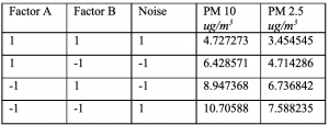
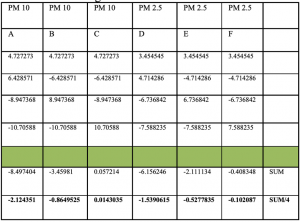
Table 2. Calculating variation in the factors

Key:
Factor A&D= window up/down
Factor B&E= inland/coastal highway
Factor C&F= “noise” or background
Window up= +1 Window down=-1
Inland highway=+1 Coastal highway=-1

Focusing on our factorial experiment, we found out several interesting significance in our results. First and foremost, a factorial experiment, 2 or more factors are examined through different combinations of what factors are present and which are not. When a factor is present, it is given a plus or positive sign. When a factor is not present, it is given a minus or negative sign (ex: window up=+1 and window down= -1). Our combinations and data recorded for PM 2.5 and PM 10 are shown in Table 1 and implementing the factorial method is shown in Table 2. After the combinations are put in place, you sum each column, as shown by the second to last row. Then, you divide that sum by four, shown by the last row.
The main takeaway here is what we see in the last row of bolded numbers, also known as response factors or how significant each factor is on affecting the chosen data (in this case, PM levels). The most significant factors are the ones with numbers farthest from zero.
For PM 10, that is factor A, or window up/down, since the value is -2.124351: the largest number of PM 10 values out of the three first columns (-2.124351, -0.8649525, 0.0143035). This means that A has the most significant impact on the average value of PM 10.The negativity of this value suggests that the values of PM 10 are on a window down are on average 2.124351 ug/m^3 lower than what we measure on window up. The least significant factor is the one with the number closest to zero; for PM 10 (first three columns), that factor is C or “noise”, due to the value equating 0.0143035 (we can assume then that it has little to no effect on the PM 10 levels).
For PM 2.5, the most significant factor is factor D, or window up/down, since the value is -1.5390615: the largest number of PM 2.5 values out of the second set of three columns (-1.5390615,-0.5277835,-0.102087). This means that D has the most significant impact on the average value of PM 2.5. The negativity of D’s value, -1.5390615, tells us that the PM 2.5 levels that we measure on window down are on average 1.5390615 ug/m^3 lower than what we measure with window up. In contrast, factor “F”, or noise, is not too far off from zero (-0.102087), so we can assume that it has little to no effect on the PM 2.5 levels.
In summary, the most significant factors for PM 2.5 and PM 10 are having the windows up or down and the least significant factors for both PM’s are “noise” or the background, which is expected since background measurements exist as a baseline of the lowest values we record. Therefore, we found that windows play a larger role than the location of measurements being taken since the window up versus down had a greater response factor than that of coastal versus inland highways.
Note that the factorial experiment was not the only method we chose in analyzing our data, but it is that which I have chosen as the most interesting. Since our hypothesis revolved around the difference in location and the wind playing a factor in PM levels, while windows up/down would have less of a role in PM data, it is fascinating that our hypothesis was rather disproved as windows resulted in being more significant of a factor than location of measurements.

Unanswered Questions

Some questions that remained unanswered is whether or not speed of the car played a role in the PM levels that were recorded. Another unanswered question is whether the influx and variation of traffic, such as surplus amounts of trucks passing us, had an effect on the PM levels. Furthermore, the time and season our measurements were taken also leaves questions on whether recording PM levels, say in the summer time or at night time as opposed to day time, will showcase different results and the extent of contrasting those results are to our experiment. We also have to consider whether our method of holding the sensor could have been altered and possibly play a larger role in effecting our sensor measuring PM levels.

References

https://www.jstor.org/stable/pdf/20486064.pdf?refreqid=excelsior%3A381dab07050076fcfb74645db01b3a21
Environmental Chemistry by Colin Baird and Michael Cann